Producing high resolution animations of high-dimensional data with tourr
Introduction
GGobi and its R wrapper package (RGgobi) are excellent for exploratory data analysis. One difficulty, however, is showing other people what you’ve found with these tools. To be fair, the focus of the tool is probably more individual – showing a single user where interesting patterns and correlations might lie – so that the user can then evaluate the truth of those patterns with a more quantitative method. I imagine the GGobi developers still see other quantitative methods or simpler graphs as the principal means of communicating to others what you’ve discovered in GGobi.
That said, the graphics GGobi produces are very attractive and impressive. It could be very useful to be able to publish and distribute them to others. If you search for GGobi videos, you will find many screen captures. These are very straight-forward to make, but they suffer from framerate and resolution limitations. They also suffer from reproducibility; it would be impossible to reconstruct the same tour paths over again if you only wanted to make a simple change to the colors, for instance. Screen captures also take some work – cropping for only the window of interest, trimming the resulting video to remove breaks when you had to adjust the parameters – to get looking professional. For these reasons, I recommend another direction: using the R-based tourr package to produce paths that can be rendered into an image sequence and subsequently encoded into a video.
Procedure
- Use savehistory() to build each subpath.
- If necessary, you can manually add or modify subpaths, but remember to run the subpath through orthonormalise() or orthonormalise_by() afterward so that you can be sure to provide valid input.
- Combine all subpaths with the abind package. abind(), as opposed to rbind and cbind, concatenates 3-dimensional matrices.
- Add attributes such as $data and the object’s $class to the new combined path object from one of the subpaths.
- Render the entire path into a sequence of PNG files.
- Encode the PNG sequence into a video with a tool like avconv.
Modifications for aesthetics
I needed to hack into the tourr package in order to achieve the aesthetics I had in mind. In display_xy() I added a new axes representation similar to the “center” option called “highlight”. This option removes the line segments, makes the axes labels unabbreviated and their font larger, and additionally sets the opacity and size of the text based on distance from the origin. The size/opacity adjustment really cleans up the video, making it feel less cluttered. In retrospect it would probably have been cleaner to just implement a new display function for these changes, which I plan to do next.
Example
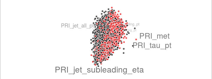
Here is an example animation based on roughly 68,000 training data points from the Higgs Boson Machine Learning challenge. I selected just the primary/raw/non-derived features and colored each entry by the training label (signal or noise). For this animation I combined 5 tourr paths:
- A little tour to start with simple 1x1 comparisons
- Random grand tour to give a sense of the number of dimensions
- Guided tour based on the LDA pursuit projection index, started from the default projection
- Guided tour based on the LDA pursuit projection index, restarted from a random projection
- Guided tour based on the LDA pursuit projection index, restarted from a random projection
Here is the R code:
library(tourr)
library(abind)

#load training data from Higgs ML competition
higgs <- read.csv('training.csv')
higgs$color <- "#000000AA"
higgs$color[higgs$Label == 's'] <- "#EA0102AA"

#simply remove cases with any missing data
#  NB: this is a boring way to handle missing data,
#  much better to use some sort of imputation,
#  but this is just for demonstration
higgs[higgs==-999] <- NA
higgs <- higgs[complete.cases(higgs),]

#set random seed so that we can reproduce the same video later
set.seed(1)

#construct the tourr paths
p1 <- save_history(data=higgs[,15:31], tour_path=little_tour(2), max_bases = 16)
p2 <- save_history(data=higgs[,15:31], tour_path=grand_tour(2), max_bases = 10)
p3 <- save_history(data=higgs[,15:31], tour_path=guided_tour(lda_pp(higgs$Label),max.tries=3))
p4 <- save_history(data=higgs[,15:31], start=basis_random(17,2), tour_path=guided_tour(lda_pp(higgs$Label),max.tries=3))
p5 <- save_history(data=higgs[,15:31], start=basis_random(17,2), tour_path=guided_tour(lda_pp(higgs$Label),max.tries=3))

#join the separate paths into a single 3D array with abind
combined.path <- abind(p1,p2,p3,p4,p5)

#add the attributes from the first path (or any of them) to the
attributes(combined.path)$data <- attributes(p1)$data
attributes(combined.path)$class <- "history_array"
render(higgs[,15:31], planned_tour(combined.path), display_xy(pch=21,col=higgs$color,axes="highlight",full.labels=T), "png", "higgs-%04d.png", width=720, height=480, apf=1/35, frames=4000)
And here is the resulting video: